A Practical Dive Into the Mechanics of the Gaussian PDF
Published on Mar 26, 2026 • Updated on Apr 30, 2026
 Credit: benjaminec/Getty Images
If you have invested considerable time in statistics, you have inevitably relied on Gaussian Probability Density Function (whether for A/B testing or any broader inferential task). But have you ever taken the time to think about how we arrived at that expression?
This article walks through the mathematical foundation of the Normal PDF, starting with the events that not only ignited it but its evolution in modern application of statistics.
1. The Discovery of Ceres
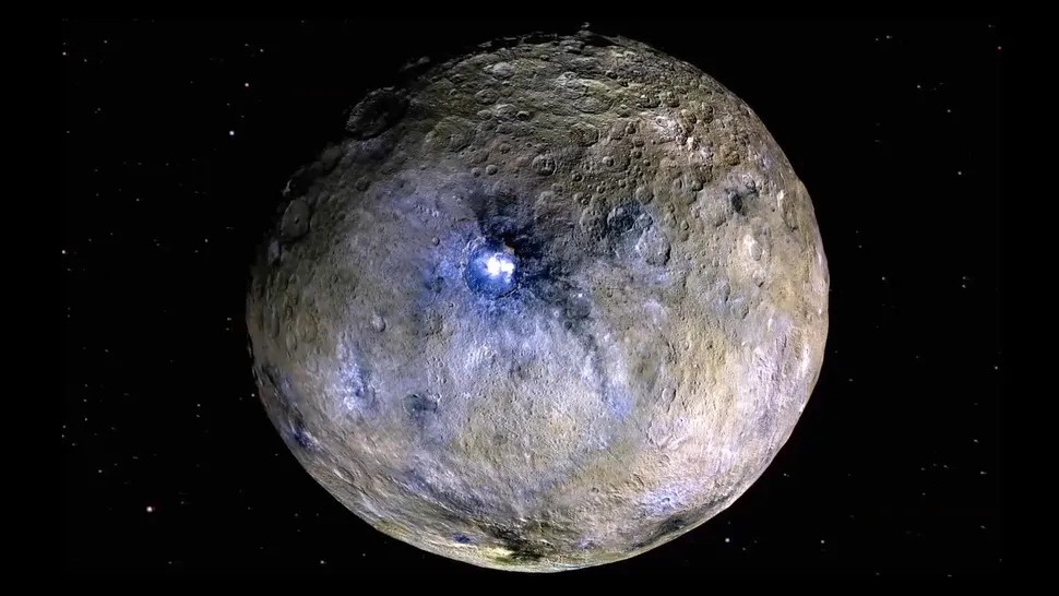 Ceres Image Capture (Credit: NASA)
On January 1, 1801, what was then announced as the new planet Ceres (later classified as the first asteroid and now a dwarf planet) was discovered by Giuseppe Piazzi at the Palermo Astronomical Observatory, in Sicily. This discovery occurred before Piazzi was invited to join the “Celestial Police” (a group of twenty-four elite astronomers tasked with finding a suspected “missing” planet between Mars and Jupiter). While their collective efforts led to several other astronomical breakthroughs, the predicted planet itself remained elusive.
Piazzi initially mistook Ceres for a comet while searching for the 87th star in the catalog of the French astronomer Abbé de Lacaille. He tracked the object twenty-four times before his final sighting on February 11th. By the time his observations were published, in September of that year, Piazzi had become convinced that its slow, uniform movement suggested something far more significant than a mere comet.
As he wrote to his contemporary, the astronomer Barnaba Oriani: “I have presented this star as a comet, but owing to its lack of nebulosity, and to its motion being too slow rather than uniform, I feel in the heart that it could be something better than a comet, perhaps. […]”.
A major problem had emerged though: by then, Ceres’ position had changed so much that it was lost in the glare of the sun. As it re-emerged, other astronomers found it nearly impossible to relocate the object based on Piazzi’s limited data. That is, until a young German mathematician named Carl Friedrich Gauss decided to get involved.
2. Gauss and the Recovery of the Lost Planet
On December 7, 1801, Ceres was finally recovered. The German astronomer Franz Xaver von Zach was the first to catch a glimpse of it, and by December 31, he had confirmed its planetary nature thanks to the method developed by the then twenty-four-year-old German prodigy. Gauss tackled the problem of few and highly imprecise observations by synthesizing two revolutionary ideas: Maximum Likelihood and Best Estimation.
a) The Maximum Likelihood Estimation
Let \(M_1,\quad M_2,\quad M_3,\quad \ldots,\quad M_n\) be several independent observations of Ceres. Let also \(x\) be the actual or “true value” of Ceres’ position. The errors of these observations can be expressed as:
Gauss defines a probability density function, \(L,\) that describes how likely any error of measurement is as \(\Phi(\Delta_i)\). To find the total probability of seeing this specific set of observations, we take the product of their individual probabilities (recalling from probability theory that \(P(A_1 \cap A_2 \cap \ldots \cap A_n) = P(A_1) \cdot P(A_2) \cdot \ldots \cdot P(A_n)\), for \(n\) independent events):
Since it is mathematically simpler to work with sums than products, we transform the Likelihood Function into a Log-Likelihood Function:
Now, a crucial question arises: which value of \(x\) maximizes this joint probability to give us the most accurate estimation of Ceres’ position? In calculus, this is solved by finding where the derivative equals zero:
This equation defines the Maximum Likelihood Estimation (MLE). By applying the chain rule, we can expand this to:
b) The Axiom of the Mean
For any set of observations, Gauss postulates that the arithmetic mean is the most natural candidate for the “true” value. In his own words: “[…] if any quantity has been determined by several direct observations, made under the same circumstances and with equal care, the arithmetical mean of the observed values affords the most probable value, if not rigorously, yet very nearly at least, so that it is always most safe to adhere to it”.
Mathematically, this “Axiom of the Mean” identifies the best estimate \(x\) as:
This assumption carries a powerful implication. If \(x\) is the average of all \(M_i\), then the sum of the individual deviations must logically nullify itself:
2.1 Solving the Functional Equation
Gauss then compares equations [2] and [3]. In this comparison, he asserts that for both conditions to hold simultaneously for any set of observations, the ratio of the two terms must be a “constant quantity”, which we will call \(k\):
By separating the variables and integrating both sides:
Recall that \(\Phi(\Delta)\) represents the likelihood of an individual measurement. Thus, from [4] we can infer that the maximum probability is such that the squared errors are minimized. Let \(\exp(c) = A\) and \(\frac{1}{2} k = -h^2\), where \(h\) is what Gauss termed the “measure of precision” (here, the constant \(k\) is set to negative since the likelihood of the observations, \(\Phi(\Delta)\), must decay for large errors). And given that the total probability must sum to 1, we solve for \(A\):
Switching to polar coordinates, and “[…] by the elegant theorem first discovered by Laplace […]”, we have that:
* Expand to see the full demonstration
Since \(x\) is a dummy variable, the key to evaluating this integral is to consider its square (why? Because \(e^{-x^2}\) has no elementary antiderivative; that is, direct integration is impossible). This allows us to treat the product of two independent integrals as a single double integral over the Cartesian plane:
To solve this, we transform the integral into polar coordinates, where \(x^2 + y^2 = r^2\), where \(x = rcos(\theta)\) and \(y = rsin(\theta)\). Additionally, we have that in Cartesian coordinates the differential area element, \(dA = dx dy\), becomes \(det(J) dr d\theta\). The (distortion) factor \(det(J)\) accounts for the change from Cartesian to polar coordinates from the substitution rule of multiple integrals (which states that, when using other coordinates, the Jacobian determinant of the coordinate conversion formula has to be considered).
The Jacobian matrix of a vector-valued function \(f:\mathbb{R^n} \implies \mathbb{R^m}\) is the \(m \times n\) matrix of all first-order partial derivatives:
As we have seen, the polar coordinate map is \(\mathbf{f}(r, \theta) = (x \quad y) = (rcos\theta \quad rsin\theta)\). For our concrete case, the Jacobian is:
Hence, the determinant is:
That is how the differential area \(dA = dx dy\) becomes \(dA = rdr d\theta\). With this arrangement, the limits of integration then change from the entire \(xy\)-plane to \(r \in [0, \infty)\) and \(\theta \in [0, 2\pi)\):
Since the integrand does not depend on \(\theta\), we can separate the integrals:
Let us denote \(I_\theta\) as the integral dependent on \(\theta\) and \(I_r\) its radial counterpart:
The result of the angular component, \(I_\theta\), is straightforward:
For \(I_r\) we use \(u\)-substitution. Let \(u = -r^2 \implies -\frac{1}{2}du = rdr\), which implies:
It is worth noting though that the double integral trick and the polar coordinates conversion approach was proposed later by Poisson, as Laplace’s starting point was Euler’s integral.
Therefore, this results in:
We can now write equation [4] in terms of \(h\) as originally written in Theoria Motus as:
Substituting this back into our Likelihood Function (Equation [1]), we arrive at the total Likelihood:
This result proved that maximizing the likelihood of the observations is equivalent to minimizing the sum of squared errors — the mathematical core of what we now call Ordinary Least Squares (OLS).
The presented framework was robust enough to recover Ceres from the void. However, its true potential was only beginning to be realized; the Gaussian PDF would soon move from the stars to nearly every field of human inquiry.
3. Beyond the Stars: a new perspective on Precision
Over a decade later, Gauss revisited and refined his ideas from Theoria Motus, solidifying the OLS method in his 1823 work, Theoria Combinationis. The most remarkable shift in this later work was his formal derivation of the “mean error”, \(m\). Gauss realized that “[…] taken from \(x = -\infty\) to \(x = +\infty\) (the mean square of \(x\)) seems most appropriate to generally define and quantify the uncertainty of the observations. Thus, given two systems of observations which differ in their likelihoods, we will say that the one for which the integral \(\int xx\varphi(x)dx\) is smaller is the more precise” (Note: He here used \(x\) and \(\varphi(x)\) to denote the error and its probability, which we have referred to as \(\Delta\) and \(\Phi(\Delta)\) throughout this article, respectively).
Additionally, this work allowed him to move beyond his earlier “Axiom of the Mean”. In Theoria Motus, he had assumed the arithmetic mean was the most probable value to justify the distribution; in Theoria Combinationis, he proved it. He demonstrated that the mean is the Best Linear Unbiased Estimator (BLUE). This was a massive leap as he showed that regardless of the underlying distribution of the errors, the mean remains the mathematically superior choice for minimizing variance.
3.1 Deriving the Mean Square Error
We begin by expressing the mean square of the error as the expected value of \(\Delta^2\):
Substituting \(\Phi(\Delta)\) from our previously derived function, we obtain:
We solve this using Integration by Parts (IBP), where \(\int udv = uv - \int vdu\). Let:
- \(u = \Delta \implies du = d\Delta\).
- \(dv = \Delta e^{-h^2\Delta^2}d\Delta \implies v = \int\Delta e^{-h^2\Delta^2}d\Delta\).
Before moving to the IBP, let us first find the solution for \(v\) by setting \(w = -h^2\Delta^2\), which implies:
Plugging these in, the mean square error becomes:
The first term in \(m^2\), which we now denote as \(t,\) vanishes. At \(\Delta \to \pm\infty\), it takes the indeterminate form \(\infty \cdot 0\). Rewriting as a ratio:
This now becomes \(\frac{\infty}{\infty}\), so L’Hôpital’s rule applies. Differentiating numerator and denominator with respect to \(\Delta\):
Since both \(|\Delta|\) and \(e^{h^2\Delta^2}\) diverge, the denominator grows without bound in both limits, giving \(t = 0\). This leaves us with:
3.2 From Measure of Precision to Standard Deviation
We can now rewrite our error function in Equation [4] in terms of \(m\):
This formulation was a game-changer, allowing the method to transcend its astronomical roots. A closer look at this mathematical sequence reveals that what Gauss termed the “mean error,” \(m\), is precisely what we recognize today as the Standard Deviation.
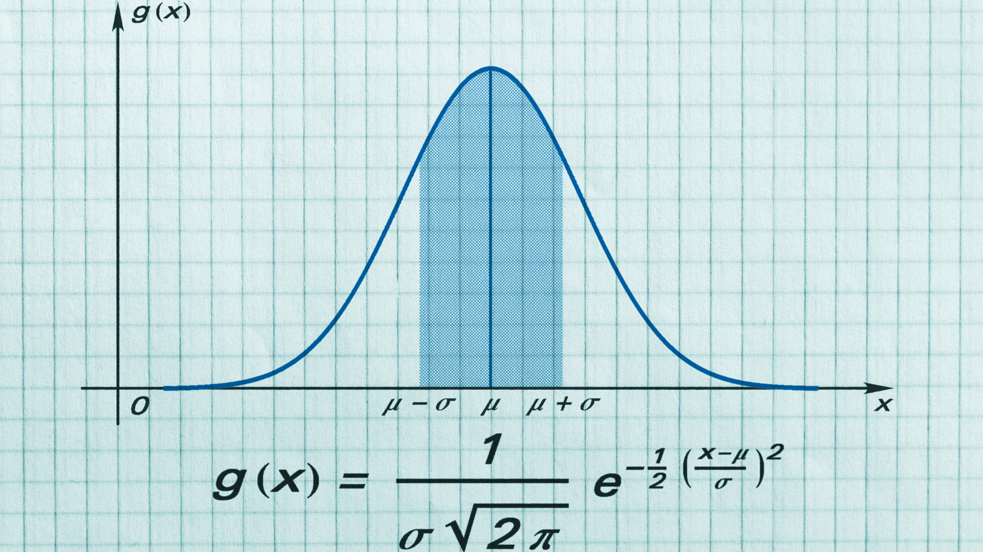
The term Standard Deviation was famously coined by Karl Pearson in 1893, who, building on the work of Francis Galton, Walter Weldon, and others, extended Gauss’s contributions into the biological sciences. Hence, by expressing the error \(\Delta\) as \((x - \mu)\), where \(\mu\) is the arithmetic mean and \(x\) represents the individual observations, and substituting Pearson’s \(\sigma\) for \(m\), we arrive at the modern Normal Distribution Probability Density Function:
And this is the exact expression used today to model an array of phenomena, from the natural sciences to marketing analytics and modern Machine Learning applications like Gaussian Naive Bayes. What once began as a mathematical device to recover Ceres has become one of the most fundamental tools for understanding and quantifying uncertainty.
References
⤶ Back to all posts
